Blog Archive
Labels
- Best Excel Books (1)
- Best Excel Website (1)
- Dynamic Chart in Excel (1)
- Excel (1)
- Excel Books (1)
- Excel Shortcuts (1)
- Excel Tips (1)
- ISERROR Macro (1)
- Selection of only visible cells in Excel (1)
- VBA (2)
- VBA Books (1)
Disclaimer
Hi All, I came across a wonderful macro where you can change the formula of a give cell or selection if it gives you error values like #DIV!, #Value! etc. This is a very effective macro for files or excel models where you have to deal with lot of formulas and calculation that affects your output. Below are the steps for the file:
Save this file on your desktop and then open it
Open the model where you want to use the ISERROR formula
Highlight the range you want to use the formula
Hit Ctrl+e to run the macro for ISERROR formula
If you want to undo please use Ctrl+z
Please note this will work for only formulas where cell reference is done and not for the below:
#DIV/0! Text
50 Not a cell reference formula
#VALUE! comments
Below is the macro code attached in the file:
Type SaveRange
Value As Variant
Address As String
End Type
Public OldWorkbook As Workbook
Public OldSheet As Worksheet
Public OldSelection() As SaveRange
Sub If_Is_Error()
'
' If_Is_Error Macro
' Changes =x to =if(iserror(x),"",x)
'
' Keyboard Shortcut: Ctrl+e
'
Dim ManualCalc As Boolean
If Application.Calculation = xlCalculationManual Then ManualCalc = True
Application.Calculation = xlCalculationManual
Application.ScreenUpdating = False
Dim x As String
' Save current values for later undoing
ReDim OldSelection(Selection.Count)
Set OldWorkbook = ActiveWorkbook
Set OldSheet = ActiveSheet
i = 0
For Each cell In Selection
i = i + 1
OldSelection(i).Address = cell.Address
OldSelection(i).Value = cell.Formula
Next cell
' make each cell is_error="" if it is a formula
For i = 1 To UBound(OldSelection)
If Len(Range(OldSelection(i).Address).Formula) = 0 Then GoTo skip
If Left(Range(OldSelection(i).Address).Formula, 1) <> "=" Then GoTo skip
x = Right(Range(OldSelection(i).Address).Formula, Len(Range(OldSelection(i).Address).Formula) - 1)
x = "=IF(ISERROR(" & x & "),0," & x & ")"
Range(OldSelection(i).Address).Formula = x
x = 0
skip:
Next i
'Return claculation to automatic if required
If ManualCalc = True Then Application.Calculation = xlCalculationManual Else Application.Calculation = xlCalculationAutomatic
' If ManualCalc = True Then MsgBox "Calculation left on manual." & Chr(10) & "Press F9 to calculate sheet"
Application.ScreenUpdating = True
' Specify Undo
Application.OnUndo "Undo the IsError macro", "UndoIsError"
ManualCalc = 0
End Sub
Sub UndoIsError()
On Error GoTo Problem
Application.Calculation = xlCalculationManual
Application.ScreenUpdating = True
' Make sure the correct workbook and sheet are active
OldWorkbook.Activate
OldSheet.Activate
' Restore saved formulae
For i = 1 To UBound(OldSelection)
Range(OldSelection(i).Address).Formula = OldSelection(i).Value
Next i
Exit Sub
Problem:
MsgBox "Can't undo"
End Sub
Link for download:
http://www.esnips.com/doc/01ebaaa2-2b7d-4300-9fdc-ad01f06bb864/ISERROR-macro
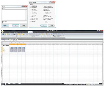
How to avoid selection of range in excel that are grouped/hidden and only select the visible ranges.
We often come in situation where we have a range of data say quarterly reviews with annual reviews of sales. In such cases mostly the quarterly data is grouped/hidden to show that they are easily recognized separately from the annuals figures. However they is a problem when we want to copy and paste the annual data for some other calculation. In this case if we copy paste we would see the whole of quarterly and annual data selected together instead of only annual data. Therefore to avoid this we have a solution.
Step 1. Group all the quarterly data as shown below. Use ALT+D+G+G to group for a selected rage and then click on the + sign on the top of the sheet to hide the quarterly data.
Step 2: Select the data you want to copy for annuals, in this case let’s say all of the data. After selection use the ALT+ Semicolon (;) on the key board. This will only highlight the selected ranges which are visible. Alternatively you can use Function Key F5, this will popup the Go To window. Then click on “Special” on the Go To window and you will see a list of radio button to select from. Use the “Visible cells only” and click OK.

Step 3: Now once you have the highlighted range you can copy paste which will only paste the annuals value.
Hi Guys,
Here is a list of websites which I am sure you all Excel VBA user like. Please share more websites if you think is useful. Please leave you comments as well.
1. http://www.exceltip.com/
2. http://www.mrexcel.com/articles.shtml
3. http://www.cpearson.com/Excel/Topic.aspx
4. http://groups.google.com/group/excel-macros/topics?hl=en&pli=1
5. http://xl.barasch.com/xlvbaa.htm
6. http://www.ozgrid.com/
7. http://www.vertex42.com/
8. http://www.familycomputerclub.com/
9. http://www.vbaexpress.com/portal.php
10. http://www.youtube.com/user/ExcelIsFun
11. http://www.functionx.com/vbaexcel/index.htm
12. http://www.xlmacros.com/
Hi Guys,
Below are the list of few Excel Books that you might find useful:
1) Learn Excel 97 through Excel 2007 From MrExcel - 377 Excel Mysteries Solved
2) Excel 2007: Beyond the Manual
3) Charts and Graphs for Microsoft Office Excel 2007
4) Work with formulas and functions in Microsoft Office Excel 2007
5) Pivot Table Data Crunching for Microsoft Office Excel 2007
6) Excel 2007 Power Programming with VBA
7) Microsoft Excel 2003 Programming Inside Out
8) VBA and Macros for Microsoft Excel 2007
9) Wrox Excel 2007 VBA Programmer's Reference
10) Professional Excel Development: The Definitive Guide to Developing Applications Using Microsoft Excel and VBA
More to Come......
How to link quickly any cell reference in Excel sheets.
Here are the steps:
1) Copy the range you want to link to the other sheet.
2) Copy
3) Go to the destination sheet or cell/range where you want to create the link. Right Click and select Paste Special and then click on "Paste Link" option given below the popup window. ( or use ALT+ E + L)


